Section 30

Skaling

One coupling exponent repairs the scaling laws

Listen to this chapter

Paper: Skaling: Chinchilla’s Exponents Meet Kaplan’s Coupling — Videau et al. (FAIR at Meta), 2026

The frontier chapters so far rebuilt the models. This last one rebuilds the ruler. Every budget decision in this explainer’s second half leaned on the scaling laws of chapter 14 and chapter 16, and in 2026 a team at FAIR showed that the standard formulation has a structural blind spot. Their fix, the Skaling law (pronounced exactly like “scaling”), adds a single parameter, and that one parameter changes both how well loss can be predicted and how cheaply the prediction can be bought.

Where the additive law cracks

Chinchilla’s law models the reducible loss as a sum of independent terms: one that shrinks with model size $N$ , one that shrinks with training tokens $D$ , plus an irreducible floor $E$ . A sum is a strong structural claim. It says model size and data never interact: mathematically, the mixed derivative $\partial^2 L / \partial N \partial D$ is exactly zero, whatever exponents you fit.

The paper’s opening figure shows what that assumption costs. Fit the Chinchilla law to a dense grid of 404 trained models and look at the signed prediction error at each $(N, D)$ point:

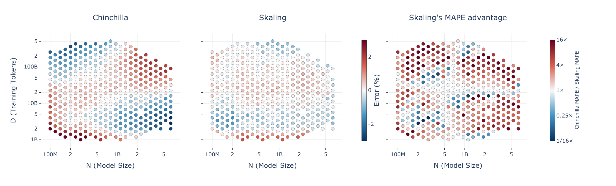
Three hexbin panels: Chinchilla's fitted error forms a saddle pattern growing toward the grid corners, Skaling's error stays near zero everywhere, and a ratio panel shows Skaling more accurate at 76% of configurations — Figure 1 from Skaling: Chinchilla’s Exponents Meet Kaplan’s Coupling (Videau et al., 2026), arXiv 2608.07222. Reproduced under CC BY 4.0.

The interior of the grid is fine. The corners are not: errors of several percent, with opposite signs in opposite corners, exactly the saddle pattern you would expect when an interaction term has been left out. And the corners are not exotic territory. Data-scarce giants and heavily over-trained small models are precisely the regimes where frontier planning happens.

Asking the loss surface directly

Before proposing a fix, the authors interrogate the loss surface itself, estimating its derivatives numerically from the trained grid. The first-order structure looks reassuringly separable: the marginal derivatives decay as clean power laws in their own variable, with only weak dependence on the other. But the decisive test is the mixed derivative. Any additive law forces it to zero; the measured one is non-zero across the entire grid, follows its own power-law decay, and is predominantly negative: growing model and data together lowers the loss by more than the sum of growing each alone. The loss surface contains a synergy that no additive formula can represent.

One exponent to couple them

The fix is minimal. Keep Chinchilla’s two interpretable inner terms, but raise their sum to a single free outer exponent $k$ :

L(N, D) = \left(\frac{A}{N^{\alpha}} + \frac{B}{D^{\beta}}\right)^{k} + E

At $k = 1$ this is the Chinchilla law, term for term. For $k \neq 1$ it reinstates the coupling that Kaplan’s original 2020 form had, without Kaplan’s drawback of tying the two decay rates together. Because the Chinchilla law is nested inside it, the Skaling law can only depart from the additive fit when the data demand it: on datasets whose surface really is nearly additive, the fitted $k$ comes back close to 1 and nothing changes.

On the two grids the paper studies, the data do demand it. The fitted coupling lands at $k \approx 0.31$ – $0.45$ , stable across cross-validation folds, and prediction error (MAPE) drops by 1.5–3× across interpolation and every extrapolation regime. The most dramatic gains are exactly where the additive law was worst: on the authors’ own training grid, far-extrapolation error falls from 5.17% to 0.70%. A nine-parameter competitor law does not close the gap, which is the telling detail: the win comes from the right inductive bias, not from extra knobs.

Try the coupling yourself. The explorer below plots the fitted Skaling surface and lets you drag $k$ back toward 1 (the Chinchilla assumption), with the synergy it erases measured live:

The Skaling explorer: one exponent bends the surface

Loss vs training tokens for three model sizes under L = (A/N^α + B/D^β)^k + E. Dashed curves are the additive law (k = 1). Drag k.

N = 300MN = 1BN = 6.4Bsame size, k = 1

Coupling exponent k = 0.41· in the paper's fitted range (0.31-0.45)

Synergy at N = 1B, D = 30B: doubling both cuts loss by 0.092; the two single-axis gains sum to 0.089 → extra +0.003 from scaling together. A sub-unit k makes the whole worth more than the sum of its parts, matching the negative mixed derivative measured on real loss surfaces.

Parameters are the paper's fitted values on the Farseer grid (A = 290, α = 0.32, B = 6000, β = 0.39, E = 0.03, k = 0.41). Sliding k with the other parameters held fixed is a schematic: in a real fit every parameter refits, and on nearly-additive datasets the fitted k itself comes back close to 1.

Fit the law from the cheap edges

The second contribution turns the better functional form into a cheaper experimental recipe. A conventional scaling study sweeps a full $N \times D$ grid, and the compute is dominated by its most expensive corner: the biggest models trained the longest. But look at the Skaling form’s limits. Train long enough and the loss isolates the model-size term; scale the model enough and it isolates the data term. Each axis of the law can be pinned down from runs where the other variable is merely held fixed, and those runs can be cheap.

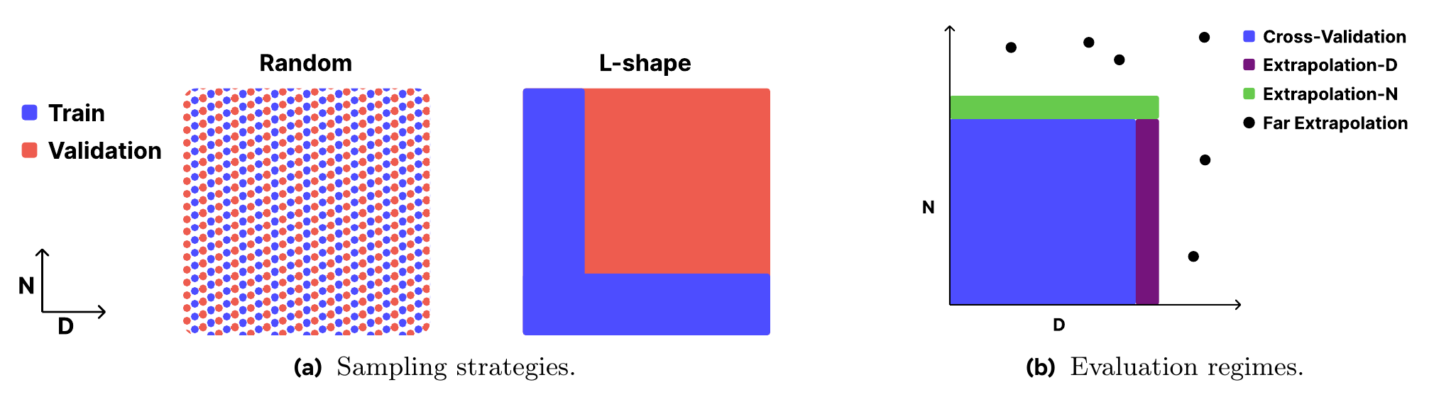
Left: random sampling scatters train and validation points across the full N-by-D grid, while the L-shape grid trains only the low-compute edges. Right: evaluation regimes showing interpolation, extrapolation in N, extrapolation in D, and far extrapolation — Figure 4 from Skaling: Chinchilla’s Exponents Meet Kaplan’s Coupling (Videau et al., 2026), arXiv 2608.07222. Reproduced under CC BY 4.0.

This L-shape grid uses roughly 10× less compute than the full sweep. Fitted on it, the Skaling law still matches or beats a full-grid Chinchilla fit; the Chinchilla law itself degrades badly under the same restriction (far-extrapolation error blowing out from 5.17% to 14.63% on one grid, against Skaling’s 1.15%). The functional form and the sampling strategy are a package: only a law that bends correctly toward the boundaries can be anchored by the boundaries.

What it changes at the frontier

The practical stakes are allocation. Frontier labs typically lock a token-to-parameter ratio and scale along it (this explainer’s model chapters are full of exactly such locked recipes), so the paper tests the operational question directly: refit every law on cheap runs only and predict the most expensive run of each recipe. Skaling is the best global law in every regime, its error never exceeding 0.9%, while the additive law is weakest precisely in the compute-optimal band that matters most.

The two laws also disagree about where the optimum moves. On the paper’s largest dataset, the Chinchilla fit says the optimal tokens-per-parameter ratio stays essentially flat as compute grows; the Skaling fit (and model-free gradient estimates, which agree with it) says the ratio drifts downward, compounding to roughly a 10× disagreement one order of magnitude beyond the fitted data. On the authors’ second grid the drift points the other way. The honest summary, and the paper is careful to make it: coupling changes large-scale allocation, but the direction of the change depends on the data and architecture, so it has to be measured, cheaply, which is what the L-shape recipe is for.

Chapter 16’s twenty-tokens-per-parameter rule was never a law of physics, and now the formula it came from has a successor. That is the right note for this explainer’s last paper: in pre-training, even the instruments are still improving. The recap now pulls the whole story together.