Attention Is All You Need
The transformer, from a training lens
Paper: Attention Is All You Need — Vaswani et al., 2017
We’ve built the training machine in the abstract. Now we meet the architecture it actually trains: the transformertransformerA neural-network architecture introduced in "Attention Is All You Need" (2017), built from stacked self-attention and feed-forward layers.See in glossary →, introduced in Vaswani et al.’s 2017 paper Attention Is All You Need. Every model in the rest of this explainer is a transformer. This chapter recaps it from a training point of view: what the forward pass computes, and therefore what backprop has to flow through.
The problem it solved
Before 2017, the best sequence models were recurrent (RNNs, LSTMs). They processed text one token at a time, each step depending on the last. That sequential dependency was fatal for training at scale: you couldn’t parallelize within a sequence, so GPUs sat idle. The transformer’s headline contribution was to replace recurrence with attention, which processes all positions at once. As the authors put it, it could be “trained for as little as twelve hours on eight P100 GPUs”. And, more importantly for us, its parallelism is exactly what later let training scale to thousands of GPUs and trillions of tokens.
It’s worth being precise about one historical point: the original transformer was a translation model, trained supervised on sentence pairs. It was not yet a pre-trained language model. The next three chapters (GPT-1, BERT, GPT-2) are the story of taking this architecture and pointing it at the self-supervised next-token (and masked-token) objectives from our foundations. But the architecture is the shared substrate, so we start here.
Self-attention, from the training side
The heart of the transformer is self-attentionself-attentionAttention where the queries, keys, and values all come from the same sequence, so each position can gather information from other allowed positions in that sequence.See in glossary →. Each token’s vector is projected into three vectors by learned weight matrices: a queryqueryA vector asking “what am I looking for in other tokens?”. Computed per token, used to score against keys.See in glossary → , a keykeyA vector saying “what I represent”. Compared against queries to compute attention scores.See in glossary → , and a valuevalueA vector representing the content actually mixed into the output when a token gets attended to.See in glossary → . The output for each token is a weighted sum of all the values, where the weights come from comparing that token’s query to every key:
The dot productdot productA single number summarizing how aligned two vectors are. To compute a · b: multiply matching components and add the results. Positive means they point partly together, zero means they are at right angles, and negative means they point partly apart; what that means for the data depends on how the vectors were learned.See in glossary → scores how much each token should attend to each other token; dividing by (the scaled dot-productscaled dot-product attentionsoftmax(QKᵀ / √d_k) · V — the canonical attention formula from “Attention is All You Need”.See in glossary →) keeps those scores from growing with dimension and saturating the softmaxsoftmaxFunction that turns any vector into a probability distribution (positive, sums to 1) by exponentiating and normalizing.See in glossary →; the softmax turns each row into attention weights; multiplying by mixes the values accordingly. The compute-dominant parts of attention are matrix multiplications, with a softmax and other elementwise operations around them. That structure is highly parallel and maps well to GPUs; gradients flow back through the learned projection matrices ().
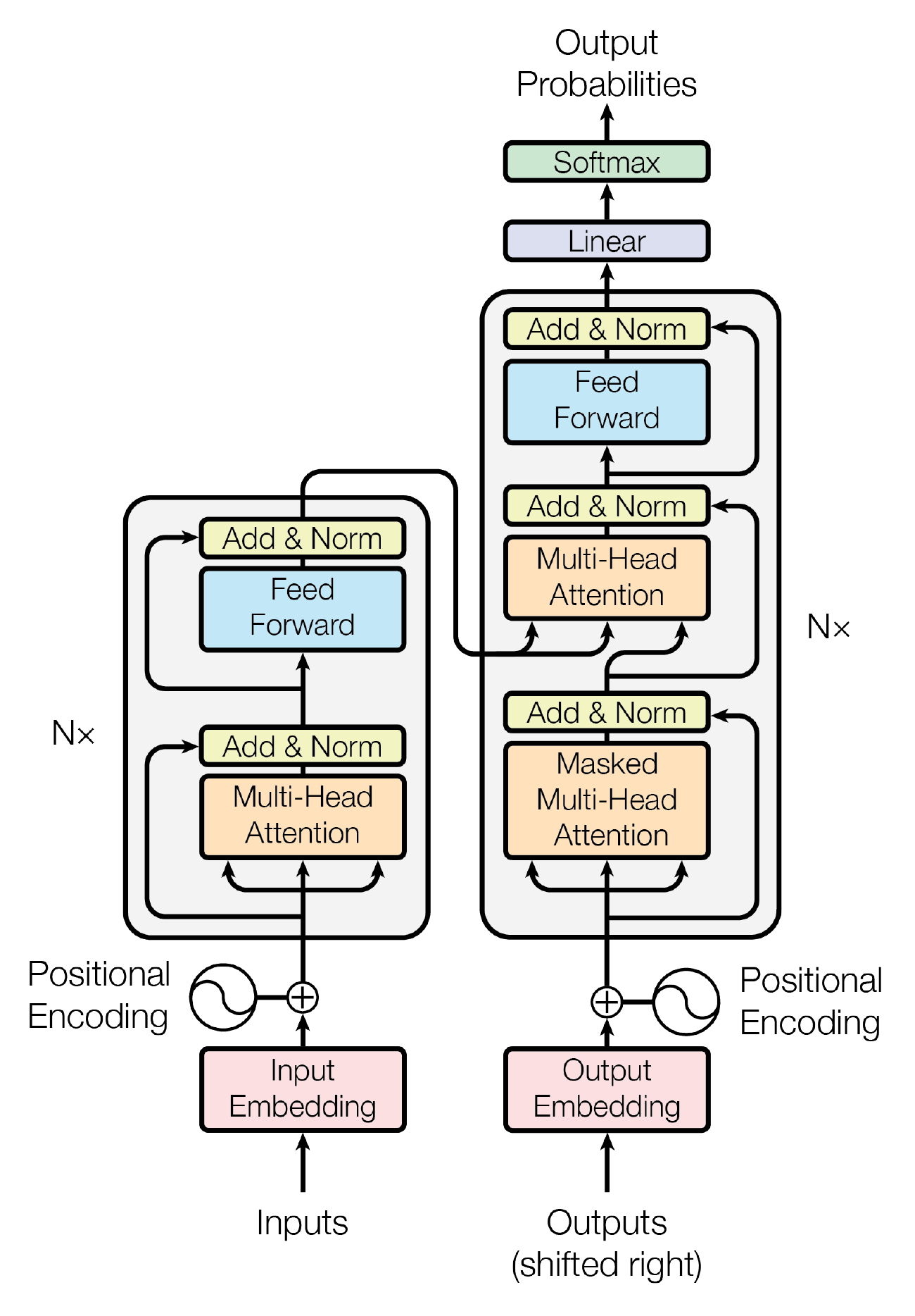
Figure 1 from Attention Is All You Need (Vaswani et al., 2017), arXiv 1706.03762.
Multi-head attention
A single attention pattern can only express one notion of “who attends to whom.” Real language needs many at once: agreement, coreference, syntax. Multi-head attentionmulti-head attentionRunning several attention operations ("heads") in parallel, each with its own learned projections, so the layer can track many kinds of relationships at once, then concatenating their outputs.See in glossary → runs several attention operations in parallel, each with its own projections into a smaller dimension (), then concatenates and projects the results. The original used heads with , keeping total compute the same as one full-width head. From a training view, each head is just more learnable matrices, all differentiated together.
The pieces that make depth trainable
Attention alone isn’t the whole block. Three supporting ingredients are what let you actually stack many layers and train them:
- A position-wise feed-forward networkMLPMulti-Layer Perceptron — a stack of dense (matrix-multiply + nonlinearity) layers applied per-token. The transformer’s feed-forward block.See in glossary → (two linear layers with a nonlinearity between, inner dimension in the base model) processes each token independently after attention. This is where much of the model’s raw capacity (and parameter count) lives.
- Residual connectionsresidual connectionoutput = x + f(x). Lets gradients flow through deep stacks and means each block adds a refinement rather than rewriting.See in glossary → wrap each sub-layer: the output is . These give gradients a direct path backward through the whole stack, which is the single most important trick for training deep networks.
- LayerNormLayerNormLayer Normalization — rescales each token's activation vector to zero mean and unit variance (then applies learned scale/shift), stabilizing training. RMSNorm is the cheaper modern variant.See in glossary → normalizes activations around each sub-layer, keeping their scale in check.
Position, and the original training recipe
Because attention is order-agnostic (it’s a weighted sum, blind to sequence position), the transformer adds positional encodingspositional encodingInformation added to embeddings so the model knows where each token sits in the sequence.See in glossary → to the embeddings, originally fixed sinusoids of different frequencies. (Learned position embeddings worked about as well; modern models use rotary positions, which we’ll meet with Llama.)
The training recipe itself is a useful checkpoint against our foundations chapters. It’s all there, in miniature:
- Optimizer: Adam with , .
- Schedule: linear warmupwarmupStarting training with a tiny learning rate and ramping it up over the first few thousand steps, to avoid blowing up the still-random early model.See in glossary → for 4,000 steps, then inverse-square-root decay, the original of the warmup-then-decay pattern we now take for granted.
- Regularization: dropoutdropoutA regularizer that randomly zeroes a fraction of activations during training, forcing the network not to rely on any single unit. Common in early models; large modern pre-training often uses little or none.See in glossary → of 0.1 and label smoothinglabel smoothingSoftening the one-hot target so a little probability mass is spread over all other tokens. It slightly worsens perplexity but discourages overconfidence and often improves downstream quality.See in glossary → of 0.1.
- Data: WMT 2014 translation pairs, tokenized with BPEBPEByte-Pair Encoding — the most common tokenization algorithm. It merges frequent byte pairs into tokens.See in glossary → (a ~37k shared vocabulary).
The base model was 65M parameters; the “big” model 213M. Tiny by today’s standards, but the architecture scaled essentially unchanged to a thousand times that size. That scalability is the whole reason the next decade happened. The first team to point this architecture at self-supervised pre-training was OpenAI, with GPT-1.